Standard Deviation, Beta, Alpha, and Sharpe Ratio Explained for Advisors

Last updated: February 2026

Most advisors can define standard deviation, beta, and the Sharpe ratio if pressed. Fewer can explain what those metrics actually tell a client about their portfolio, where each metric breaks down, and when one measure matters more than another. The gap between knowing the definitions and applying the metrics in practice is where fund evaluation gets interesting, and where most surface-level explanations stop short.

Standard Deviation: What Volatility Actually Measures

Standard deviation is the most widely reported measure of investment risk. It quantifies how much a fund’s returns vary around their average over a given period. A fund with an annualized standard deviation of 15% has experienced a wider dispersion of returns than a fund with a standard deviation of 8%. Morningstar, Lipper, and most fund screeners calculate standard deviation using 36 monthly return observations, updated quarterly.

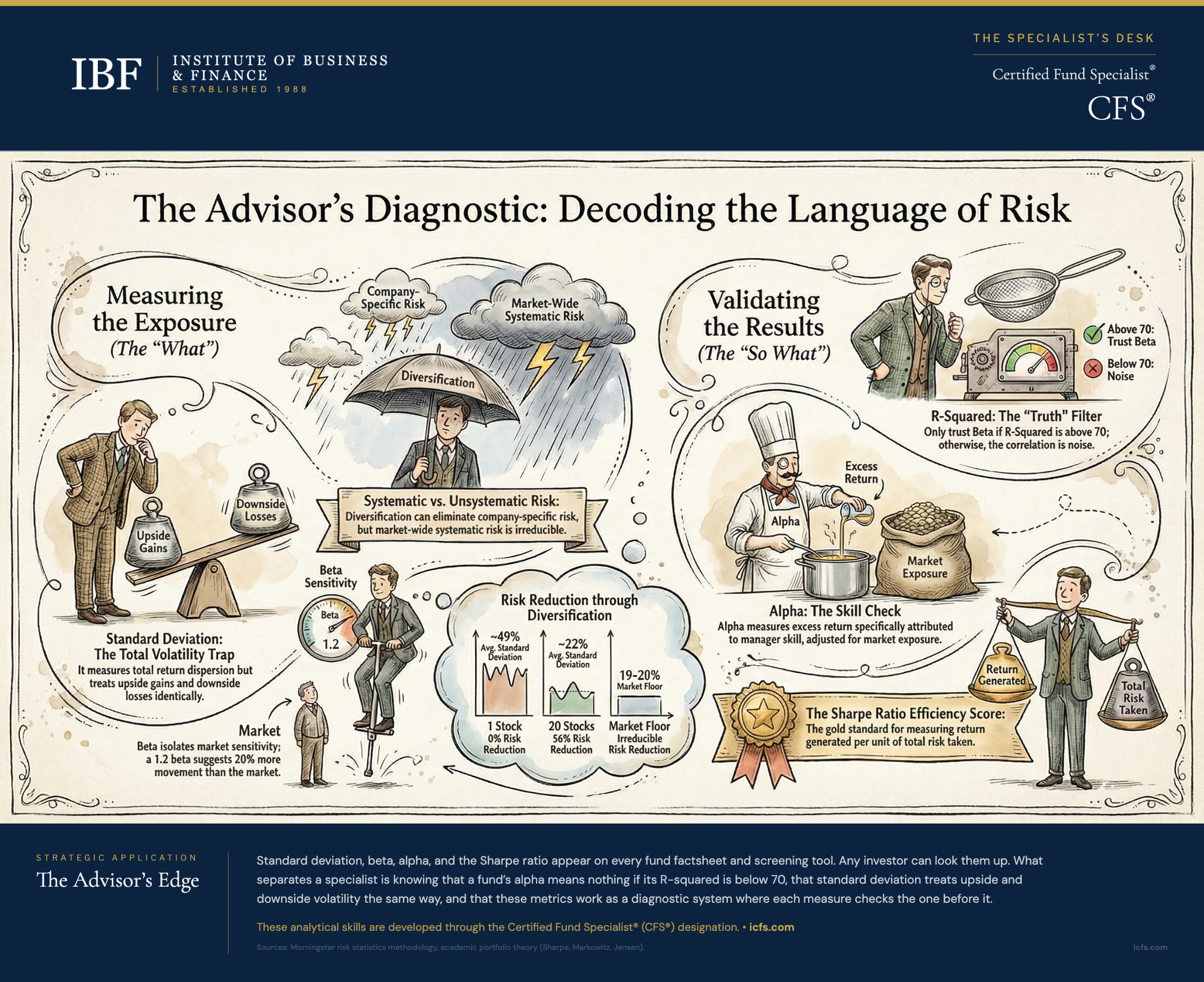
The metric is intuitive in concept but frequently misunderstood in practice. Standard deviation treats upside and downside volatility identically. A fund that shoots above its average by 5% in one month and drops below by 5% the next registers the same standard deviation as a fund that grinds steadily upward with occasional sharp drops. For clients who experience loss far more acutely than they appreciate gain (a well-documented behavioral pattern), standard deviation can understate the risk that actually keeps them awake at night.

Despite that limitation, standard deviation remains the foundation of portfolio risk measurement for a practical reason: it connects directly to the two categories of risk that drive every diversification conversation.

Systematic and Unsystematic Risk: The Two Risks Inside Every Portfolio

Every portfolio’s standard deviation reflects a combination of two distinct risk types. Understanding the difference between them is not academic. It determines whether adding a position to a portfolio actually improves it or simply adds noise.

Systematic risk (also called market risk) arises from forces that affect all securities in a market: interest rate changes, recessions, geopolitical events, inflation, and broad shifts in investor sentiment. This risk cannot be eliminated by holding more stocks. A portfolio of 500 U.S. equities is just as exposed to a Federal Reserve rate increase as a portfolio of 20. Systematic risk is the risk investors are compensated for bearing.

Unsystematic risk (also called company-specific, diversifiable, or idiosyncratic risk) arises from factors unique to an individual company: a product recall, a management shake-up, a patent dispute, or a key customer loss. This risk can be eliminated almost entirely through diversification.

The research quantifying this relationship is among the most replicated in portfolio theory. A foundational study by Elton and Gruber (1977) measured how the standard deviation of a stock portfolio changes as holdings increase. A single stock had an average standard deviation of approximately 49%. Moving to just four stocks dropped that figure to roughly 30%, a 40% reduction in total risk. By 20 stocks drawn from different sectors, standard deviation settled near 22%, eliminating about 56% of the original risk. Beyond 100 stocks, additional diversification produced almost no further reduction.

The remaining risk after full diversification is systematic risk. For a well-diversified U.S. equity portfolio, that floor sits near 19-20% standard deviation. This is the irreducible volatility that comes from being in the stock market at all.

The practical takeaway for fund evaluation: when comparing two equity funds with different standard deviations, the relevant question is whether the difference reflects genuine systematic risk exposure (which the market compensates) or undiversified company-specific risk (which it does not). A sector fund concentrated in energy stocks and a total market fund may have similar average returns over time, but the sector fund’s higher standard deviation reflects unsystematic risk that the investor is not rewarded for taking.

Beta: Measuring Market Sensitivity

If standard deviation measures total risk, beta isolates the systematic component. Beta quantifies how sensitive a fund’s returns are to movements in a benchmark, almost always the S&P 500 for U.S. equity funds.

The S&P 500 has a beta of 1.0 by definition, whether the market is in a bull run or a crash. A fund with a beta of 1.2 is expected to move 20% more than the S&P 500 in either direction. A fund with a beta of 0.7 is expected to capture 70% of the market’s movement up and down.

Beta varies considerably across industries. Utility stocks, with their stable revenue streams and regulated pricing, have historically carried betas in the 0.5-0.7 range. Technology and energy companies, whose earnings are more sensitive to economic cycles and commodity prices, tend to land in the 1.1-1.3 range. REITs and large banks historically cluster near 0.8, reflecting their income-oriented nature combined with interest rate sensitivity.

The metric has clear practical value for portfolio construction: an advisor building a portfolio for a client who needs reduced market sensitivity can tilt toward lower-beta holdings, while an advisor building for long-term growth in a tax-advantaged account might accept higher-beta exposure for its historically higher expected return.

But beta has important limitations that advisors should recognize. First, beta is backward-looking. It is calculated from historical returns, typically over three to five years. Research by Fama and French (1992) demonstrated that past beta is a poor predictor of future beta for individual stocks. Stock betas tend to revert toward 1.0 over time: a stock that showed a 1.5 beta in one period is likely to register a lower beta in the next. This mean reversion is less pronounced for broad fund categories than for individual stocks, but it means that a fund’s current beta should be treated as an estimate, not a guarantee, of future market sensitivity.

Second, beta only captures the linear relationship between a fund and its benchmark. A fund that uses options, leverage, or concentrated positions may respond to market movements in ways that beta does not predict. During the 2008 financial crisis, many funds with moderate betas experienced drawdowns that far exceeded what their beta would have suggested, because the correlations across asset classes spiked simultaneously.

Third, beta is only as useful as the benchmark is relevant. A fund benchmarked against the S&P 500 but invested primarily in small-cap international stocks will produce a beta that tells you very little about its actual risk characteristics. This is where R-squared becomes essential.

R-Squared: When to Trust Beta (and When to Ignore It)

R-squared measures the percentage of a fund’s return movements explained by its benchmark. It answers a simple but critical question: is this fund’s beta actually telling me something useful?

The scale runs from 0 to 100. An R-squared of 95 means that 95% of the fund’s performance variation is attributable to benchmark movements. An R-squared of 30 means that only 30% of the fund’s returns are explained by the benchmark, and the remaining 70% comes from sources the benchmark does not capture.

Morningstar’s general guidance provides a practical rule of thumb. An R-squared of 70-100 indicates a strong return correlation between the fund and its benchmark, making beta a reliable indicator of market sensitivity. An R-squared of 40-70 represents average correlation, where beta provides some signal but should be interpreted cautiously. An R-squared below 40 indicates weak correlation, where the fund’s beta relative to that benchmark is essentially noise.

The practical application is immediate. Before citing a fund’s beta in a client presentation or a portfolio analysis, check the R-squared first. A large-cap blend fund tracking closely to the S&P 500 will typically have an R-squared above 90, and its beta is worth discussing. A precious metals fund with an R-squared of 12 relative to the S&P 500 has a beta that tells you almost nothing about its behavior. For that fund, standard deviation is the more appropriate risk measure, or you need to compare it against a commodity or precious metals benchmark.

R-squared is calculated as the square of the correlation coefficient between the fund and its benchmark. A fund with a correlation of 0.9 to the S&P 500 has an R-squared of 81. A fund with a correlation of 0.5 has an R-squared of 25. The squaring amplifies differences: a modest drop in correlation produces a large drop in R-squared, which is why the metric is effective at separating funds whose beta you should pay attention to from those where beta is misleading.

Alpha: The Performance That Matters

Alpha measures a fund’s return in excess of what its beta-adjusted benchmark exposure would predict. It is, in theory, the purest measure of whether a manager has added value through skill.

If a fund has a beta of 1.0 and the S&P 500 returned 10% over a period, the expected return based on market exposure alone is 10%. If the fund actually returned 12%, the alpha is +2%. If it returned 8%, the alpha is -2%. For funds with betas above or below 1.0, the calculation adjusts proportionally: a fund with a 1.2 beta and a 15% return during a period when the market returned 10% has an expected return of 12% (1.2 times the market return), producing an alpha of +3%.

Alpha is the metric active managers point to when justifying their fees, and the metric index fund advocates use to argue those fees are not earned. Long-term data consistently shows that the average active fund produces negative alpha after expenses. The SPIVA Scorecard reports that over 15-year periods, roughly 90% of active large-cap managers generate negative alpha relative to their benchmarks. That statistic is what drives the passive investing movement.

For advisors evaluating active funds, alpha requires the same R-squared check that beta does. A fund with a low R-squared relative to its stated benchmark may show large positive alpha simply because it is taking on risk the benchmark does not capture, not because the manager is skilled. True alpha, the kind that reflects genuine investment skill, requires both a positive return above what the benchmark predicts and an appropriate benchmark that actually reflects the fund’s risk exposures.

Alpha is also sensitive to the time period measured. A manager can produce strong alpha over three years through concentrated bets that happen to work, then give it all back in year four. The persistence of alpha over rolling periods is a more reliable signal than alpha measured over any single stretch.

The Sharpe Ratio: Putting Risk and Return Together

The Sharpe ratio, developed by William Sharpe (the same Nobel laureate who articulated the arithmetic of active management), combines return and risk into a single number. It divides a fund’s excess return above the risk-free rate by its standard deviation. The result tells you how much return the fund generated per unit of total risk.

A fund that returned 10% when Treasury bills yielded 2% and had a standard deviation of 16% produces a Sharpe ratio of 0.50 (the 8% excess return divided by 16% standard deviation). A fund with the same 10% return, the same 2% risk-free rate, but a standard deviation of 10% produces a Sharpe ratio of 0.80. The second fund delivered the same return with substantially less volatility, making it the superior risk-adjusted performer.

The Sharpe ratio is the standard measure for comparing funds across different risk levels. Raw returns are misleading when the funds being compared have different volatility profiles. A fund returning 15% with a standard deviation of 25% may look impressive until compared with a fund returning 11% with a standard deviation of 12%. The Sharpe ratio makes that comparison direct.

In practice, Sharpe ratios above 1.0 are considered strong over extended periods. Ratios between 0.5 and 1.0 are acceptable. Ratios below 0.5 suggest the investor is not being adequately compensated for the risk taken. Like all backward-looking metrics, the Sharpe ratio is calculated from historical data and is not a guarantee of future risk-adjusted performance, but it remains the single most useful number for answering the question “was the risk worth it?”

The ratio has one notable limitation: because it uses standard deviation (which counts upside and downside volatility equally), a fund with large positive surprises is penalized the same way as a fund with large negative surprises. For advisors working with clients who are primarily concerned about downside risk, the Sortino ratio (which substitutes downside deviation for standard deviation in the denominator) provides a more targeted measure.

How These Metrics Work Together in Practice

No single risk metric tells the complete story. In practice, advisors who evaluate funds effectively use these measures as a system rather than in isolation.

Start with standard deviation to understand a fund’s total risk. Then check R-squared to determine whether the fund’s returns are closely tied to its stated benchmark. If R-squared is high (above 70), beta becomes a reliable measure of market sensitivity and alpha provides a useful assessment of manager value-added. If R-squared is low, beta and alpha calculated against that benchmark are unreliable, and the advisor should either find a more appropriate benchmark or rely on standard deviation and the Sharpe ratio for risk assessment.

The Sharpe ratio provides the summary comparison. When choosing between two funds with similar investment objectives, the fund with the higher Sharpe ratio has delivered better compensation for the risk it took, regardless of whether that risk showed up as market sensitivity (beta) or as total volatility (standard deviation).

This layered approach also catches common evaluation mistakes. A fund with a high R-squared, a beta near 1.0, and a negative alpha is essentially an expensive index fund. A fund with a low R-squared showing impressive alpha may simply be taking risks the benchmark does not reflect, making the alpha misleading. A fund with a low Sharpe ratio despite strong raw returns is delivering those returns at a cost in volatility that may not suit the client’s risk tolerance.

The Client Conversation This Enables

Clients rarely ask about standard deviation or beta by name. They ask questions like: “Why did my portfolio drop more than my neighbor’s?” or “Is this fund worth the higher fee?” or “Should I move to something safer?” Every one of those questions has an answer rooted in these metrics.

The portfolio that dropped more may have held higher-beta funds or carried concentrated sector exposure with significant unsystematic risk. The fund charging higher fees may or may not justify them with positive alpha, and checking the Sharpe ratio provides the clearest answer. “Moving to something safer” means reducing standard deviation, which the advisor can accomplish by shifting toward lower-beta equity funds, adding fixed-income exposure, or simply ensuring the existing holdings are well diversified enough to have eliminated the unsystematic risk that earns no premium.

Framing risk metrics as tools for answering real client questions, rather than as technical definitions to memorize, is what separates professional advice from a fund fact sheet.

The Advisor’s Edge

The definitions of standard deviation, beta, alpha, and the Sharpe ratio are available in any investment textbook or online glossary. What separates professional fund analysis from basic literacy is the ability to read these metrics as a system, to recognize when a metric is misleading for a particular fund, to connect risk measurements to portfolio construction decisions, and to translate statistical concepts into language that helps clients understand why their portfolio is built the way it is. These are the analytical skills that the Certified Fund Specialist (CFS) designation develops across its two-module curriculum. For advisors looking to see how risk metrics connect to the diversification research, the Portfolio Diversification for Risk Reduction article explores how standard deviation decreases as portfolio holdings increase and why unsystematic risk earns no return premium.

Sources and Notes: The diversification and standard deviation research referenced draws from Elton and Gruber (1977) and subsequent replication studies. Beta mean reversion findings reference Fama and French (1992). R-squared interpretation guidelines follow Morningstar’s fund analysis methodology. SPIVA Scorecard data is published by S&P Dow Jones Indices and referenced in the companion article on active manager performance. Sharpe ratio interpretation benchmarks reflect commonly used practitioner standards. Industry beta data draws from NYU Stern School of Business research. Advisors should verify current risk metrics through Morningstar, Bloomberg, or their preferred data provider, as these figures are updated quarterly. This article is refreshed every 18 months or when major methodology changes occur in the referenced data sources.